반응형
* XOR
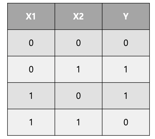
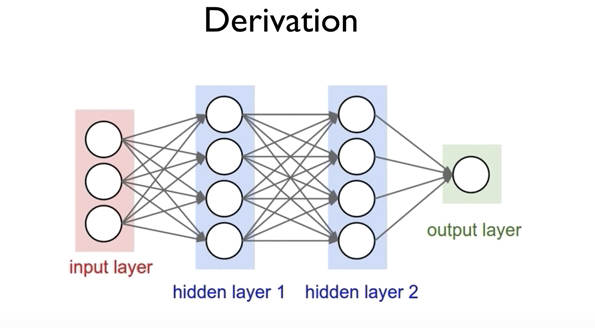
- Multiple logistic regression 으로 해결 가능 (3개의 network)
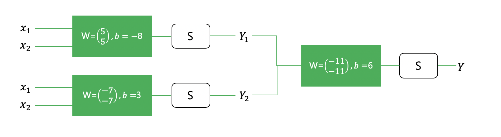
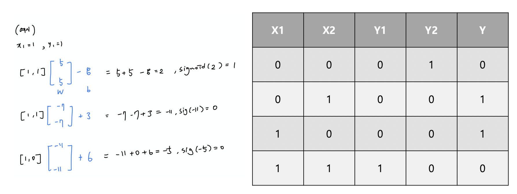
* Weight 과 bias를 행렬로 나타내어 처리 할 수 있음
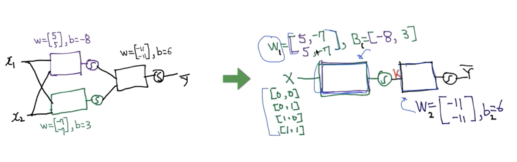
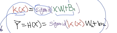
- Layers 각각의 Weight과 bias 어떻게 예측할 것인지
(W와 b의 값을 어떻게 자동적으로 학습할 수 있을지)
*G (Gradient Descent Algorithm)
x1(각각의 입력 값)이 Y에 끼치는 영향(미분값)을 알아야 예측 할 수 있음
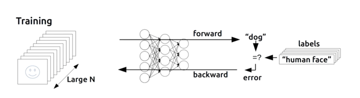
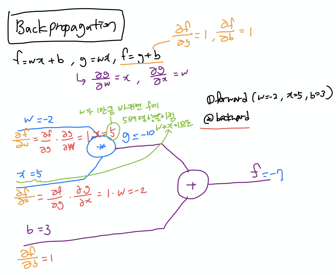
Backpropagation Algorithm
예측값과 출력값을 비교해서 cost를 backward로 보내 W,b 예측
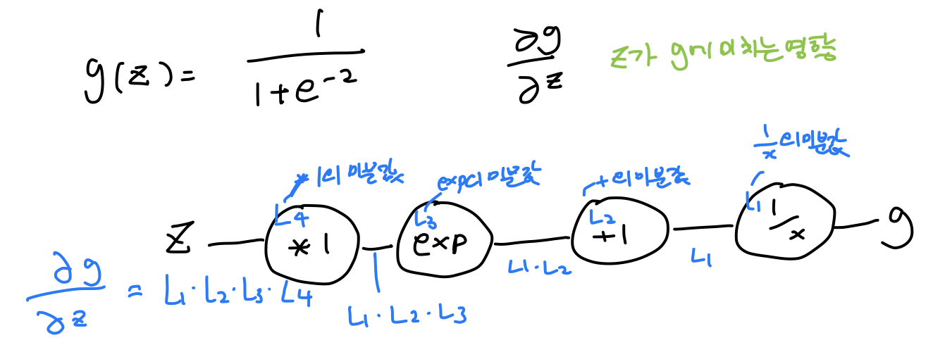
*sigmoid 미분
* 실습 - Xor layer 구성
import tensorflow as tf
import numpy as np
x_data = np.array([[0,0],[0,1],[1,0],[1,1]],dtype=np.float32)
y_data = np.array([[0], [1], [1], [0]],dtype=np.float32)
X = tf.placeholder(tf.float32)
Y = tf.placeholder(tf.float32)
#W = tf.Variable(tf.random_normal([2,1]),name='weight')
#b = tf.Variable(tf.random_normal([1]), name='bias')
#hypothesis = tf.sigmoid(tf.matmul(X,W) + b)
#layer 구
W1 = tf.Variable(tf.random_normal([2,2]), name='weight1')
b1 = tf.Variable(tf.random_normal([2]), name='bias1')
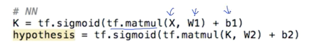
layer1 = tf.sigmoid(tf.matmul(X,W1)+ b1)
W2= tf.Variable(tf.random_normal([2,1]), name='weight2')
b2 = tf.Variable(tf.random_normal([1]), name='bias2')
#wide layer
#W1 = tf.Variable(tf.random_normal([2,10]), name='weight1')
#b1 = tf.Variable(tf.random_normal([10]), name='bias1')
#layer1 = tf.sigmoid(tf.matmul(X,W1)+ b1)
#
#W2= tf.Variable(tf.random_normal([10,1]), name='weight2')
#b2 = tf.Variable(tf.random_normal([1]), name='bias2')
hypothesis = tf.sigmoid(tf.matmul(layer1,W2) + b2)
cost = -tf.reduce_mean(Y * tf.log(hypothesis) + (1 - Y) * tf.log(1 - hypothesis))
train = tf.train.GradientDescentOptimizer(learning_rate=0.1).minimize(cost)
predicted = tf.cast(hypothesis>0.5, dtype=tf.float32)
accuracy = tf.reduce_mean(tf.cast(tf.equal(predicted,Y),dtype=tf.float32))
with tf.Session() as sess:
sess.run(tf.global_variables_initializer())
for step in range(10001):
sess.run(train,feed_dict={X:x_data,Y:y_data})
if step % 100 == 0:
print(step,sess.run(cost, feed_dict={X:x_data,Y:y_data}),sess.run([W1,W2]))
h,c,a = sess.run([hypothesis, predicted, accuracy], feed_dict={X:x_data,Y:y_data})
print("\nHypothesis: ",h,"\nCorrect: ",c,"\nAccuracy : ",a)
*실습2 - MNIST layer 구성
import tensorflow as tf
import matplotlib.pyplot as plt
import random
from tensorflow.examples.tutorials.mnist import input_data
mnist = input_data.read_data_sets("MNIST_data",one_hot = True)
nb_classes = 10
X = tf.placeholder(tf.float32,[None,784])
Y = tf.placeholder(tf.float32,[None,nb_classes])
#W = tf.Variable(tf.random_normal([784,nb_classes]))
#b = tf.Variable(tf.random_normal([nb_classes]))
#hypothesis = tf.nn.softmax(tf.matmul(X,W) + b)
#layer 구성
W1 = tf.Variable(tf.random_normal([784,28]),name='weight1')
b1 = tf.Variable(tf.random_normal([28]),name='bias1')
layer1 = tf.nn.softmax(tf.matmul(X,W1)+b1)
W2 = tf.Variable(tf.random_normal([28,28]),name='weight2')
b2 = tf.Variable(tf.random_normal([28]),name='bias2')
layer2 = tf.nn.softmax(tf.matmul(layer1,W2)+b2)
W3 = tf.Variable(tf.random_normal([28,nb_classes]),name='weight3')
b3 = tf.Variable(tf.random_normal([nb_classes]),name='bias3')
hypothesis = tf.nn.softmax(tf.matmul(layer2,W3)+b3)
cost = tf.reduce_mean(-tf.reduce_sum(Y * tf.log(hypothesis), axis=1))
train = tf.train.GradientDescentOptimizer(learning_rate=0.1).minimize(cost)
is_correct = tf.equal(tf.argmax(hypothesis,1), tf.argmax(Y,1))
accuracy = tf.reduce_mean(tf.cast(is_correct,tf.float32))
num_epochs = 15
batch_size = 100
num_iterations = int(mnist.train.num_examples / batch_size)
with tf.Session() as sess:
sess.run(tf.global_variables_initializer())
for epoch in range(num_epochs):
avg_cost = 0
for i in range(num_iterations):
batch_xs, batch_ys = mnist.train.next_batch(batch_size)
_, cost_val = sess.run([train,cost], feed_dict={X: batch_xs, Y: batch_ys})
avg_cost += cost_val / num_iterations
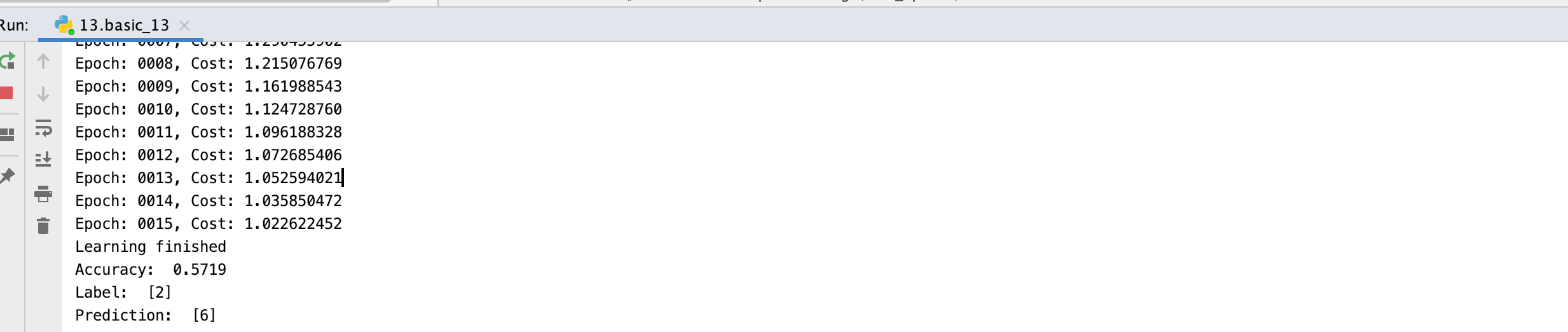
print("Epoch: {:04d}, Cost: {:.9f}".format(epoch + 1, avg_cost))
print("Learning finished")
print(
"Accuracy: ",
accuracy.eval(
session=sess, feed_dict={X: mnist.test.images, Y: mnist.test.labels}
),
)
# Get one and predict
r = random.randint(0, mnist.test.num_examples - 1)
print("Label: ", sess.run(tf.argmax(mnist.test.labels[r: r + 1], 1)))
print(
"Prediction: ",
sess.run(tf.argmax(hypothesis, 1), feed_dict={X: mnist.test.images[r: r + 1]}),
)
plt.imshow(
mnist.test.images[r: r + 1].reshape(28, 28),
cmap="Greys",
interpolation="nearest",
)
plt.show()
* Layer를 구성해서 실행시킨 결과 - accuracy 가 낮아짐
(조금 더 공부)
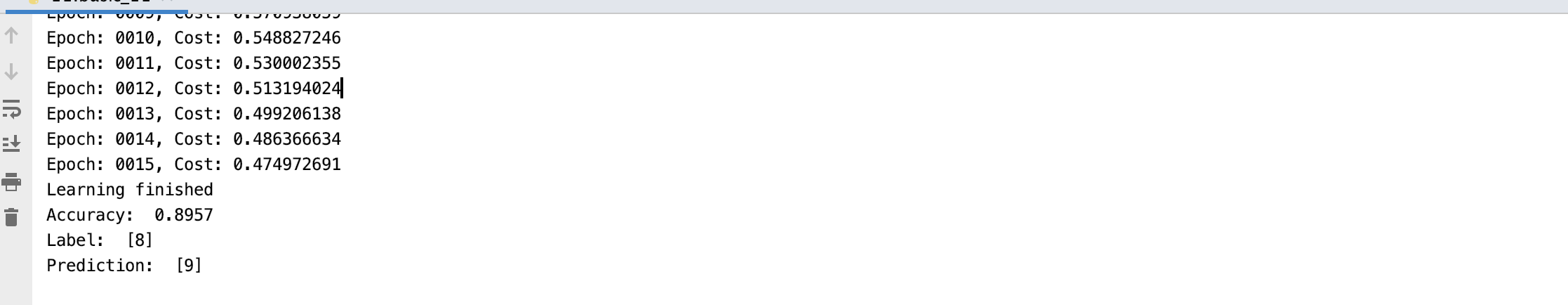
이전 MNIST 실습 결과
출처 : 모두를 위한 딥러닝
반응형
'개발자 > 모두를 위한 딥러닝' 카테고리의 다른 글
| 11. Convolutional Neural Network (0) | 2020.02.19 |
|---|---|
| 10.ReLU, weight 초기화, DropOut과 Ensemble (0) | 2020.02.19 |
| 08.Neural Network (0) | 2020.02.18 |
| 07. Application & Tips (0) | 2020.02.16 |
| 06.Multinomial classification - Softmax Classification (0) | 2020.02.14 |


