* Learning rate
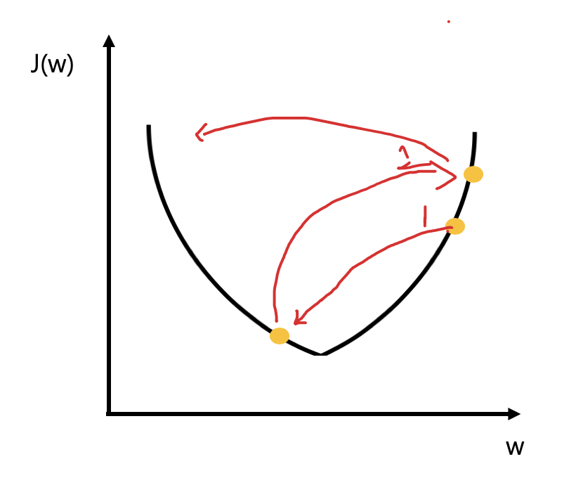
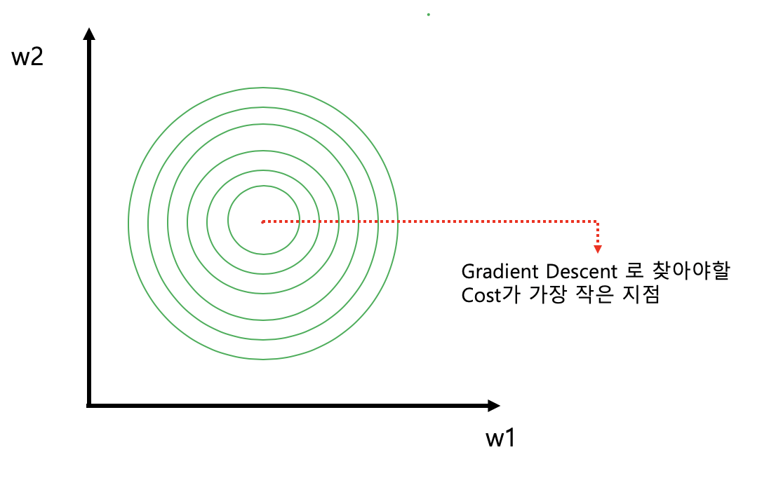
- Gradient descent : cost를 가장 작게 하는 값을 찾기 위해 사용
- learning rate 를 알맞게 정하는 것이 중요
1) Learning rate 가 너무 큰 경우 -> overshooting 발생
- cost가 점점 커지는 경우가 발생
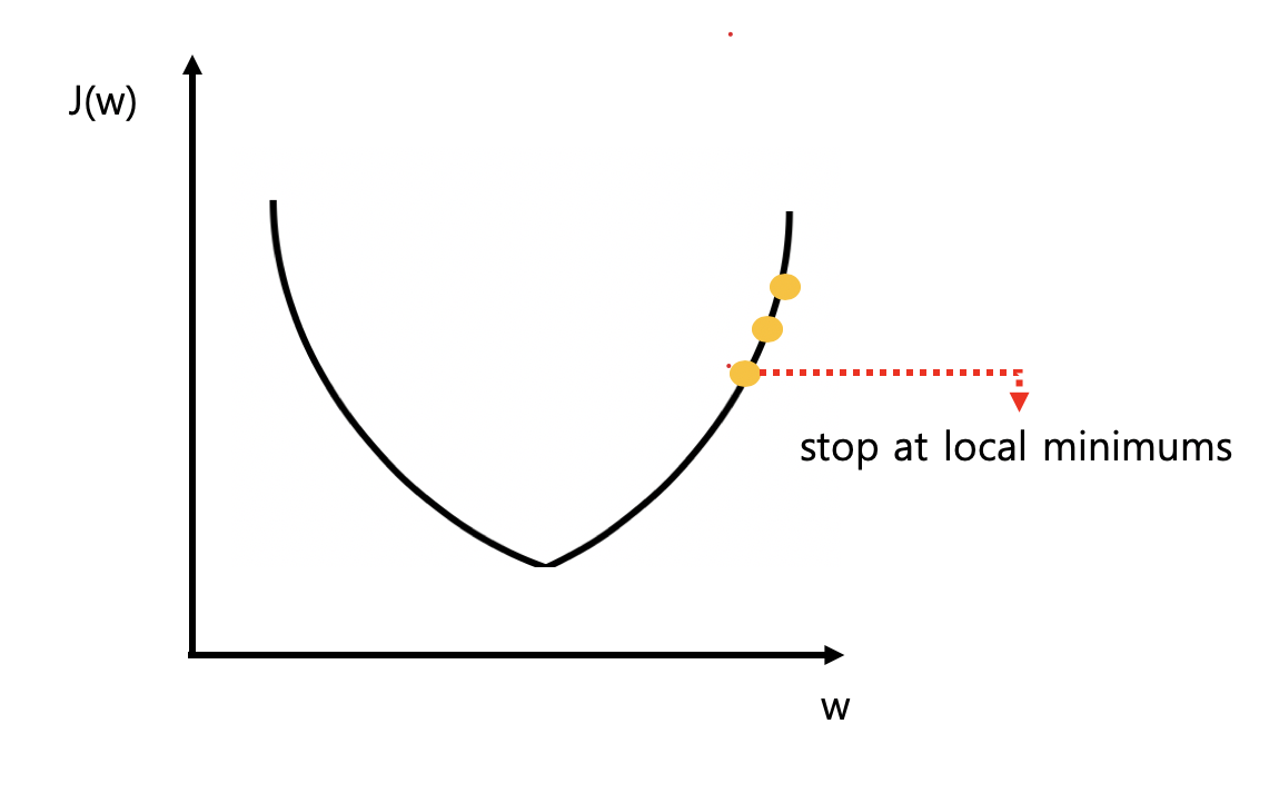
2) learning rate 가 너무 작은 경우
- local minimun에서 멈추는 현상 발생
해결방법
- learning rate는 data나 환경에 따라 달라 질 수 잇음
- 0.01로 먼저 정하고 출력해보면서 learning rate를 수정
* Data preprocessing
- pre-processing 이 필요없는 Data set
- Data pre-processing이필요 함
-> learning rate를 적합한 값으로 선택 해도 밖으로 나갈 수 있음(cost값이 커질 수 있음)
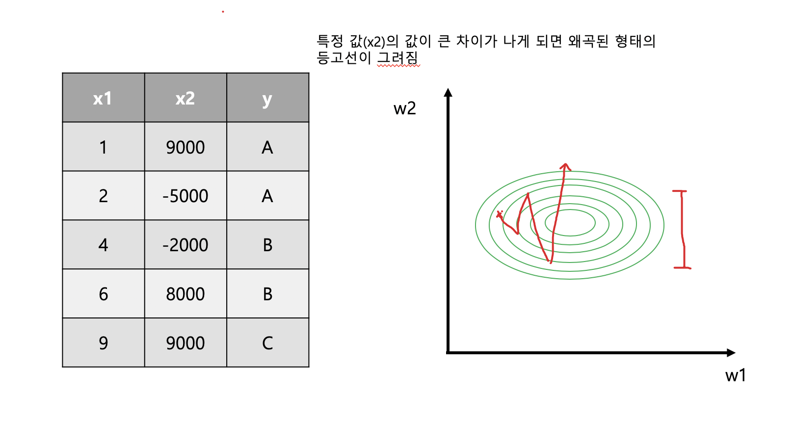
* 해결방법
- zero-centered data
- normalized data
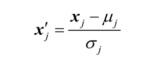
X_std[:,0] = (X[:,0] - x[:,0].mean()) / X[:,0].std()
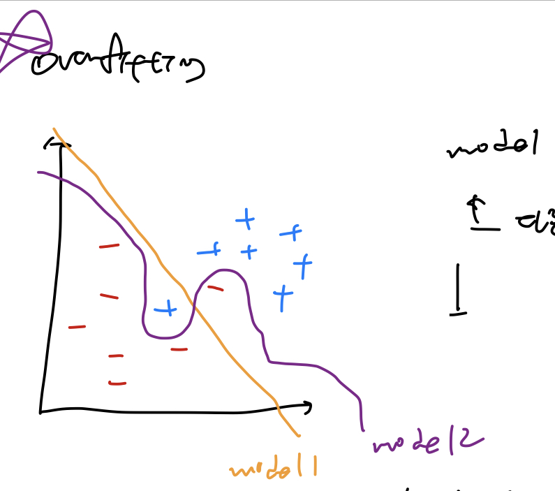
* Overfitting
- 머신러닝의 가장 큰 문제
- 학습 데이터에 너무 잘 맞는 모델을 만들어 일반적인 값을 예측할 때 오류가 생김
ex) model2는 테스트 데이터에만 적합한 모델
-> overfitting
- 해결방법
1. trainnig data를 더 많이 가진다.
2. features 개 수를 줄인다
3. Regularization -> 일반화
* Regularization
- Weigth이 적은 값을 갖게 만든다(그래프를 구부리지 말고 편다)
- cost 함수를 최소화 할 때 term을 추가
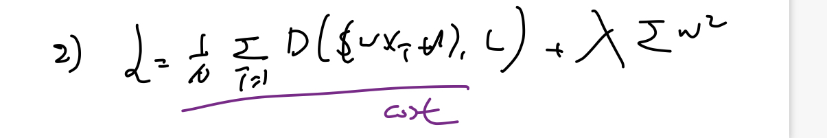
람다 : regularization strength
0 : regularization 사용하지 않음
큰값 : regularization 을 중요하게 사용
각각의 element를 제곱하여 더함
l2reg = 0.001 * tf.reduce_sum(tf.square(W))
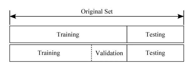
* Learning and test data sets
- Training, validation and test sets
1) Training : Model을 만들기 위해 학습 시키는 데이터
2) Validation : 알파(learing_rate), 감마(regularization)값을 조정하기 위해 사용하는 데이터
3) Test sets : Model의 정합도를 파악하기 위해 사용하는 데이터(30% 정도, 한 번만 사용)
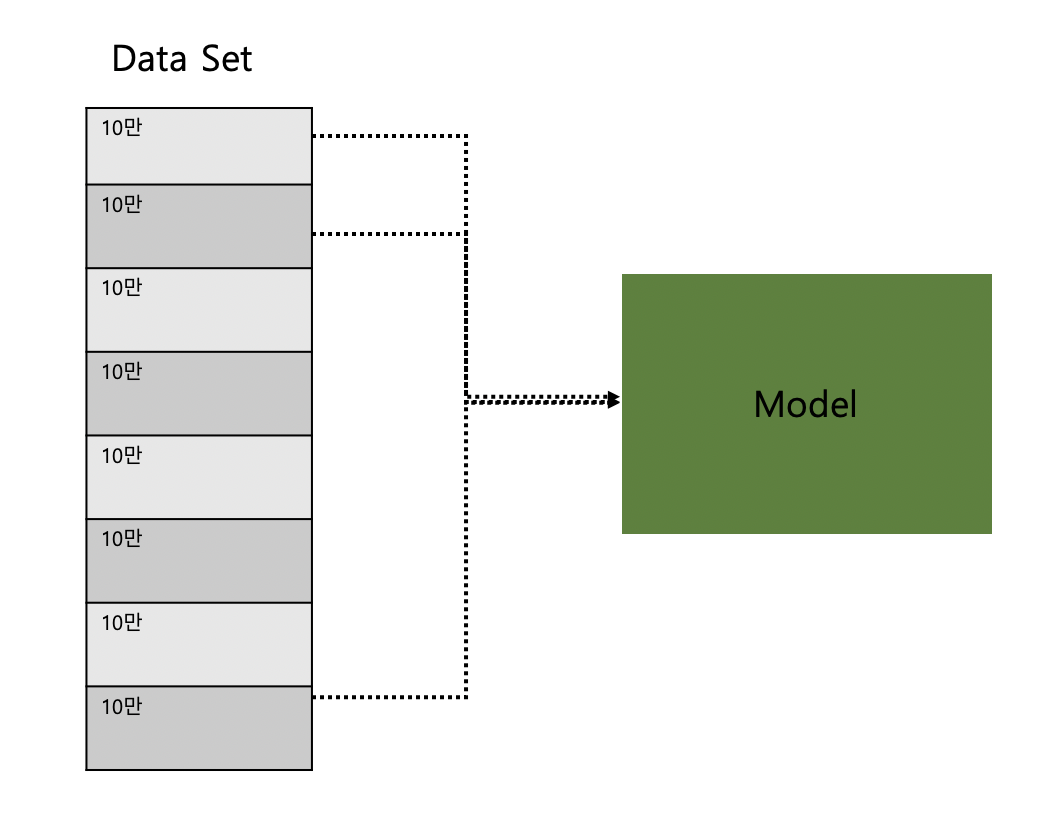
- Online learning
1. 100만개의 데이터를 10만개씩 잘라서 learning
(처음 10만개를 학습한 데이터는 모델에 남아 있음)
2. 새로 10만개의 데이터가 들어 올 때, 기존의 데이터를 처음부터 학습 시키지 않아도 됨
실습1 - training data, test data
import tensorflow as tf

x_data = [[1, 2, 1],
          [1, 3, 2],
          [1, 3, 4],
          [1, 5, 5],
          [1, 7, 5],
          [1, 2, 5],
          [1, 6, 6],
          [1, 7, 7]]
y_data = [[0, 0, 1],
          [0, 0, 1],
          [0, 0, 1],
          [0, 1, 0],
          [0, 1, 0],
          [0, 1, 0],
          [1, 0, 0],
          [1, 0, 0]]

# Evaluation our model using this test dataset
x_test = [[2, 1, 1],
          [3, 1, 2],
          [3, 3, 4]]
y_test = [[0, 0, 1],
          [0, 0, 1],
          [0, 0, 1]]

X = tf.placeholder("float",[None,3])
Y = tf.placeholder("float",[None,3])

W = tf.Variable(tf.random_normal([3,3]))
b = tf.Variable(tf.random_normal([3]))

hypothesis = tf.nn.softmax(tf.matmul(X,W)+b)
cost = tf.reduce_mean(-tf.reduce_sum(Y * tf.log(hypothesis), axis=1))
optimizer = tf.train.GradientDescentOptimizer(learning_rate=0.1).minimize(cost)

prediction = tf.arg_max(hypothesis,1)
is_correct = tf.equal(prediction, tf.arg_max(Y,1))
accuracy = tf.reduce_mean(tf.cast(is_correct,tf.float32))

with tf.Session() as sess:
    sess.run(tf.global_variables_initializer())
    for step in range(201):
        cost_val, W_val, _ = sess.run([cost,W,optimizer],
                                      feed_dict={X:x_data, Y:y_data})
        print(step, cost_val, W_val)

    print("Prediction: ",sess.run(prediction, feed_dict={X:x_test,Y:y_test}))
    print("Accuracy: ",sess.run(accuracy, feed_dict={X:x_test,Y:y_test}))
실습2 - normalized inputs : (MinMaxScaler)
import tensorflow as tf
import numpy as np

tf.set_random_seed(777)  # for reproducibility


def min_max_scaler(data):
    numerator = data - np.min(data, 0)
    denominator = np.max(data, 0) - np.min(data, 0)
    # noise term prevents the zero division
    return numerator / (denominator + 1e-7)


xy = np.array(
    [
        [828.659973, 833.450012, 908100, 828.349976, 831.659973],
        [823.02002, 828.070007, 1828100, 821.655029, 828.070007],
        [819.929993, 824.400024, 1438100, 818.97998, 824.159973],
        [816, 820.958984, 1008100, 815.48999, 819.23999],
        [819.359985, 823, 1188100, 818.469971, 818.97998],
        [819, 823, 1198100, 816, 820.450012],
        [811.700012, 815.25, 1098100, 809.780029, 813.669983],
        [809.51001, 816.659973, 1398100, 804.539978, 809.559998],
    ]
)

# normalized
xy = min_max_scaler(xy)
#print(xy)

x_data = xy[:, 0:-1]
y_data = xy[:, [-1]]

X = tf.placeholder(tf.float32, shape=[None, 4])
Y = tf.placeholder(tf.float32, shape=[None, 1])

W = tf.Variable(tf.random_normal([4, 1]), name='weight')
b = tf.Variable(tf.random_normal([1]), name='bias')

# Hypothesis
hypothesis = tf.matmul(X, W) + b

# Simplified cost/loss function
cost = tf.reduce_mean(tf.square(hypothesis - Y))

# Minimize
train = tf.train.GradientDescentOptimizer(learning_rate=1e-5).minimize(cost)

# Launch the graph in a session.
with tf.Session() as sess:
    # Initializes global variables in the graph.
    sess.run(tf.global_variables_initializer())

    for step in range(101):
        _, cost_val, hy_val = sess.run(
            [train, cost, hypothesis], feed_dict={X: x_data, Y: y_data}
        )
        print(step, "Cost: ", cost_val, "\nPrediction:\n", hy_val)
실습3 - MNIST
import tensorflow as tf
import matplotlib.pyplot as plt
import random

from tensorflow.examples.tutorials.mnist import input_data

mnist = input_data.read_data_sets("MNIST_data",one_hot = True)

nb_classes = 10

X = tf.placeholder(tf.float32,[None,784])
Y = tf.placeholder(tf.float32,[None,nb_classes])

W = tf.Variable(tf.random_normal([784,nb_classes]))
b = tf.Variable(tf.random_normal([nb_classes]))

hypothesis = tf.nn.softmax(tf.matmul(X,W) + b)

cost = tf.reduce_mean(-tf.reduce_sum(Y * tf.log(hypothesis), axis=1))
train = tf.train.GradientDescentOptimizer(learning_rate=0.1).minimize(cost)

is_correct = tf.equal(tf.argmax(hypothesis,1), tf.argmax(Y,1))

accuracy = tf.reduce_mean(tf.cast(is_correct,tf.float32))

num_epochs = 15
batch_size = 100
num_iterations = int(mnist.train.num_examples / batch_size)

with tf.Session() as sess:
    sess.run(tf.global_variables_initializer())

    for epoch in range(num_epochs):
        avg_cost = 0

        for i in range(num_iterations):
            batch_xs, batch_ys = mnist.train.next_batch(batch_size)
            _, cost_val = sess.run([train,cost], feed_dict={X: batch_xs, Y: batch_ys})
            avg_cost += cost_val / num_iterations
        print("Epoch: {:04d}, Cost: {:.9f}".format(epoch + 1, avg_cost))

    print("Learning finished")

    print(
        "Accuracy: ",
        accuracy.eval(
            session=sess, feed_dict={X: mnist.test.images, Y: mnist.test.labels}
        ),
    )

    # Get one and predict
    r = random.randint(0, mnist.test.num_examples - 1)
    print("Label: ", sess.run(tf.argmax(mnist.test.labels[r: r + 1], 1)))
    print(
        "Prediction: ",
        sess.run(tf.argmax(hypothesis, 1), feed_dict={X: mnist.test.images[r: r + 1]}),
    )

    plt.imshow(
        mnist.test.images[r: r + 1].reshape(28, 28),
        cmap="Greys",
        interpolation="nearest",
    )
    plt.show()
출처 : 모두를 위힌 딥러닝 유튜브
'개발자 > 모두를 위한 딥러닝' 카테고리의 다른 글
| 09.XOR using Neural Networks (0) | 2020.02.18 |
|---|---|
| 08.Neural Network (0) | 2020.02.18 |
| 06.Multinomial classification - Softmax Classification (0) | 2020.02.14 |
| 05.Logistic Classification (0) | 2020.02.13 |
| 04.Multi-variable linear regression (0) | 2020.02.13 |


